Legacy Metrics

Learn about defining the metrics you will use in your A/B test results

Metrics are what your experiments are trying to improve (or at least not hurt). GrowthBook has a very flexible and powerful way to define metrics.

This page describes Legacy Metrics. We highly recommend using Fact Tables to define metrics instead. Check out the docs

Conversion Types

Metrics can have different units and statistical distributions. Below are the ones GrowthBook supports:

Conversion Type	Description	Example	Default aggregation (SQL)
binomial	A simple yes/no conversion	Created Account	1/0 per unit
count	Sums conversion values per user	Pages per Visit	SUM(value) per unit
duration	How much time something takes	Time on Site	SUM(value) per unit
revenue	The revenue gained/lost	Revenue per User	SUM(value) per unit

For experiment analysis, each of these metric types uses some aggregation (often defaulting to SUM) per user and then takes an average with respect to the total number of users. In the case of SQL metrics, the only meaningful difference between count, duration, and revenue is how we render the units in the metric and experiment results pages.

Revenue Metrics are displayed in USD by default. You can change your display currency under Settings → General → Metric Settings

Query settings

For metrics to work, you need to tell GrowthBook how to query the data from your data source. There are a few ways to do this depending on your data source.

1. SQL (recommended)

If your data source supports SQL, this is the preferred way to define metrics. You can use joins, subselects, or anything else supported by your SQL dialect.

Your SELECT statement should return one row per “conversion event”. This may be a page view, a purchase, a session, or something else. The end result should look like this:

user_id	timestamp	value
123	2021-08-23 12:45:14	10
456	2021-08-23 12:45:15	5.25

Metrics can support one or more types of identifiers. The above example assumes the metric only supports a single id type called user_id, but you would add additional columns if you need to support other ones.

Non-binomial metrics

For count, revenue, and duration metrics metric types, the value represents the count, duration, or revenue from that single conversion event. In the case of multiple rows for a single user, the values will be summed together or we will use a custom aggregation that you can specify.

Therefore a count metric can really be any arbitrary metric whose value you want to sum at the user level before taking an average per variation.

If you use Segment to populate your data warehouse, the SQL for a Revenue per User metric might look like this:

SELECT
  -- Assuming you support 2 identifier types - 'user_id' and 'anonymous_id'
  user_id as user_id,
  anon_id as anonymous_id,
  received_at as timestamp,
  grand_total as value
FROM
  purchases

If you wanted to count the number of conversion rows per user, you can simply set 1 as value in your SQL query and then the default SUM aggregation will count the number of rows per user.

Binomial metrics

Binomial metrics don’t need a value column (the existence of a row means the user converted). You would only need to return the following columns, representing users and when they “converted” on this binomial metric:

user_id	timestamp
789	2022-08-23 12:45:14
111	2022-08-23 12:45:15

When we go to conduct experiment analysis, any user_id that has a conversion in the appropriate time window will be counted as a 1, while all other users will be counted as a 0. Then we can compute the proportion of users in an experiment variation who converted.

SQL Templates

We use {{Handlebars}} to compile the sql into what is actually called to your database. This allows you to create template metrics that can be copied and reused by changing the variable values associate with the metrics.

You can use the following user configurable variables within SQL templates:

• eventName - The event name associated with this metric. This can then be referenced in your sql template as {{eventName}}. Depending upon how your data is structured you can then incorporate it as part of the table name, if each event has its own table, or as part of a where clause limiting the rows returned to where a certain column equals the eventName.
• valueColumn - The column in your datawarehouse table with the metric data. This can then be referenced in your sql template as {{valueColumn}}. For example you might have {{valueColumn}} as value to extract out the value from the table.

Read more about SQL Templates and all the different variables that are available.

Denominator (Ratio / Funnel Metrics)

By default, metrics are evaluated against all users in an experiment: (# users who converted) / (# users in experiment)

You can instead choose another metric to use as the denominator.

Funnel Metrics

When the denominator is a simple binomial (conversion) metric, then it acts just like an “activation metric” in an experiment. It filters the users who are included in the analysis to those who first convert on this denominator metric.

For example, if you want to look at what percent of users checkout after viewing a cart, it can be described as % checkout / % viewed cart. This requires creating two metrics:

1. Viewed Cart - selects all users who viewed a cart
2. Viewed Cart -> Checkout - selects all users who checked out and picks Viewed Cart as the denominator.

Ratio Metrics

When the denominator is a count metric, then things are a little different. Instead of acting like a filter, we calculate both metrics and treat the value as a ratio.

• The mean is sum(metric) / sum(denominator)
• The standard deviation is calculated using the Delta method

For example, if you want to look at the Average Order Value (AOV), what you’re really looking for is total revenue / number of orders. This also requires creating two metrics:

1. Orders per User - selects the count of orders for each user
2. AOV - selects total revenue per user and picks Orders per User as the denominator.

Quantile Metrics

Quantile Metrics are available only as Fact Tables, as described here.

2. Javascript (Mixpanel only)

We query Mixpanel data sources using their proprietary JQL language based on Javascript. This allows for extreme flexibility when defining metrics.

All metrics at minimum need to specify an Event Name which must exactly match what is used in Mixpanel. You can use OR to match against multiple events. For example viewed_cart OR purchased

You can optionally add Conditions which filters the events further based on properties. For example, if Event Name is Page view, you can add a condition path = "/blog".

Count, duration, and revenue metrics have two additional steps. We first extract all event values for a user into an array and then reduce that array down to a single number, which is the final metric value for the user.

Conditions

Conditions in Mixpanel are very powerful. They consist of a Property, an Operator, and a Value. Multiple conditions are joined with an AND.

The Property can either be the name of an event property or a javascript expression. Some examples:

• amount, equivalent to event.properties.amount
• event.time
• event.properties.city + ", " + event.properties.country

The Operator is one of the following:

• equals
• does not equal
• is greater than
• is greater than or equal to
• is less than
• is less than or equal to
• matches the regex
• does not match the regex
• custom javascript

The custom javascript operator is special. The Value is a javascript expression that evaluates to either true or false (access the property value with the value variable). It lets you do arbitrarily complex filtering. For example:

value < 5 || value > 10;

For all other operators, the condition should read like an English sentence. For example:

// property operator value
country equals US

// Will render as
event.properties.country == "US"

Event Value

For count, revenue, and duration metrics, we need to know what the “value” of the event is.

The Event Value is a Javascript expression to extract a value from a raw Mixpanel event. If you are just extracting a single property as-is, you can just enter the property name as a shortcut. Otherwise, you can reference the event variable in your expression.

Here are some example Event Value expressions:

• grand_total, equivalent to event.properties.grand_total
• 1 (hard-code the value to a specific number)
• (event.properties.endTime - event.properties.startTime) / (60 * 60) (difference in hours between two unix timestamps)
• new Date(event.time).toISOString().substr(0, 10) (event timestamp in YYYY-MM-DD format)

For count metrics, you can leave Event Value blank and it will default to hard-coding the value to 1, which is perfect for when you just want to count the number of events and don’t care about specific properties.

User Value Aggregation

For count, revenue, and duration metrics, we need to know how to aggregate the event values together, in case a single user has multiple matching events.

The User Value Aggregation is another Javascript expression that reduces an array of Event Values to a single number (or null if the user did not convert). Reference the variable values in your expression. There are a few built-in helper functions:

• count(values)
• countDistinct(values)
• sum(values)
• min(values)
• max(values)
• avg(values)
• median(values)
• percentile(values, p) (p is a number between 0 and 100)

You can use your own custom expression too if you want. For example, this is the equivalent of sum(values):

values.reduce((sum, n) => sum + n, 0);

If the aggregation is left blank, we do sum(values) by default.

3. SQL Query Builder (legacy)

The query builder prompts you for things such as table/column names and constructs a SQL query behind the scenes.

We only recommend this for extremely simple metrics. Inputting raw SQL is far more flexible.

Behavior

The behavior tab lets you tweak how the metric is used in experiments. Depending on the metric type and datasource you chose, some or all of the following will be available:

What is the Goal?

For the vast majority of metrics, the goal is to increase the value. But for some metrics like “Bounce Rate” and “Page Load Time”, lower is actually better.

Setting this to “decrease” basically inverts the “Chance to Beat Control” value in experiment results so that “beating” the control means decreasing the value. This will also reverse the red and green coloring on graphs.

Capped Value

Large outliers can have an outsized effect on experiment results. For example, if your normal revenue per user $40 and someone happens to make a $5000 order, whatever variation that person is in will be much more likely “win” any experiment because that one order is an outlier.

Capping (also known as winsorization) works by ensuring that all aggregate unit (e.g. user) values are no more than some value. So in the above example, if the cap was $100, the $5000 purchase will still be counted, but the aggregated value for that user will be capped at $100 and will have a much smaller effect on the results. It will still give a boost to whatever variation the person is in, but it won’t completely dominate all of the other orders and is unlikely to make a winner just on its own. Another way to think about this is that you are slightly biasing your results by truncating large values, but you are reducing variance to prevent the outsized effect of outliers.

There are two ways to cap metric values in GrowthBook:

1. Absolute capping - if set above zero, all aggregated user values will be capped at exactly this value. For example, if the cap is $100 on total revenue per user, then after we sum all of a users orders up, any user with an aggregate sum of greater than $100 will be set to $100.

2. Percentile capping - when this is set to between 0 and 1, it uses that percentile to select a cap based on the data in your experiment so far. This cap is therefore specific to each experiment and specific to each analysis run in that experiment if new data has come in. It works like so: after we calculate the unit-level aggregate values for all units (e.g. users) during an experiment analysis, we find the specified percentile of these unit-level aggregates and then cap these aggregated values at this percentile. Using the above example, if you were to specify percentile capping with a value of 0.95, then we find the 95th percentile of total revenue per users (say this turns out to be $135). We then cap those user-level aggregates at $135.

You can additionally choose to ignore zeros, which will compute the percentile without including any user aggregated zero values. This is useful if you have a lot of zero values and you don’t want to have to fine tune the percentile to avoid setting the cap too low.

Because the percentile cap depends on the data in your experiment, it can be different from experiment to experiment, or even analysis to analysis. To find out what value was actually used for capping you can do the following: on the Experiment Results tab, click the three dot menu in the top right and select “View Queries”. Each percentile capped metric will have a column with the main_cap_value that was used to cap that metric and represents the computed percentile of unit-level aggregate values.

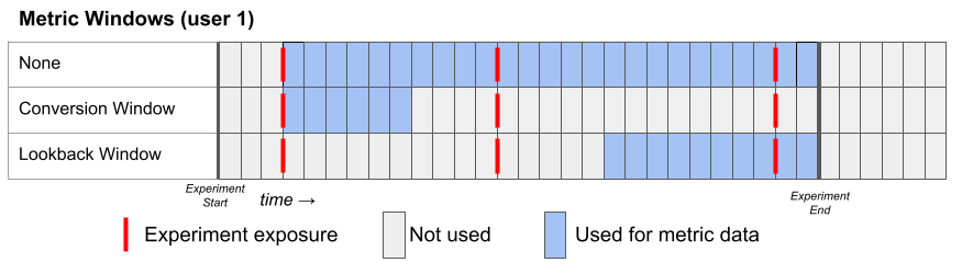
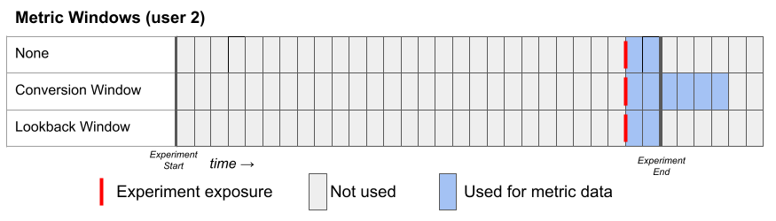
Metric Windows

When used in an experiment, we only consider rows of a Metric where the timestamp is greater than or equal to the first time the user was exposed to the experiment. In other words, if someone purchases something before seeing your experiment, it won’t be included in the analysis. This behavior is ideal for the vast majority of metrics, but you can change it with the Metric Delay setting if desired (see below).

There are three window settings one can use to configure the metric date window. Each of them defines the lower and upper date range of the metric to use for each user:

• None (default)
  • Lower bound: user’s first exposure plus the metric delay
  • Upper bound: experiment end date
• Conversion Window
  • Lower bound: user’s first exposure plus the metric delay
  • Upper bound: the lower bound + the length of the conversion window
• Lookback Window
  • Lower bound: the experiment end date minus the lookback window OR the user’s first exposure plus the metric delay, whichever is later
  • Upper bound: experiment end date

Here’s a graphical representation of these three window types for a hypothetical User 1:

Here’s a second example for a hypothetical User 2, who joins the experiment late. Notice that the conversion window can extend beyond the experiment end date.

Why might you choose one window over another?

None - The simplest. Use all data available. This is useful for using as much data associated with users in your experiment and will combine any behavior that is right after experiment exposure as well as long run behavior within the experiment time frame.

Conversion window - Conversion windows allow you to only look at events that are tied to the first exposure to an experiment. This can help if, for example, you are tracking purchases and you only want to measure the effect of an experiment in a checkout flow on purchases made soon after seeing that checkout flow. Using a conversion window can reduce the noise from user behavior not related to an experiment. However, if you set the window too short, you may not capture users that return a few days later and were influenced by the experiment.

Lookback window - Lookback windows are good for capturing long run impacts of an experiment on regular behavior like user log ins or page views. They have two main advantages:

(1) You can mitigate the novelty effect of an experiment; if you are testing a new recommendation algorithm, at first users may react a certain way to the experiment, but eventually they may adjust and so may their behavior. In these cases, you may just want to look at the last 14 days of an experiment.

(2) Lookback windows help you focus on the long run effects of an experiment. Much of experimentation is about building a better product; by focusing on impact of an experiment after it has been live for a week or two, you may get a better picture of the long run impact of launching the experiment.

Larger companies who measure long run logged in behavior want to ensure their experiments have lasting effects and often rely on lookback windows to make shipping decisions However, lookback windows may not be right if you are testing a feature on logged-out or anonymous users and are measuring simple purchase conversions or something similar. In these cases, you might end up with many logged-out users who, in the long run, simply have no metric data associated with them.

Metric Delay

Conversions within the first X hours of being put into an experiment are ignored (default = 0). This is useful for metrics like “day 2 retention”. In that case, if your underlying table reports whether a user is retained on any given day, you could set a metric delay to 24 hours.

Negative metric delays

The metric delay can also be negative to include some conversions before a user is put into an experiment. For example, a value of -2 would mean conversions up to 2 hours before will be included. You might be wondering when this would ever be useful.

Imagine the average person stays on your site for 60 seconds and your experiment can trigger at any time.

If you just look at the average time spent after the experiment, the numbers will lose a lot of meaning. A value of 20 seconds might be horrible if it happened to someone after only 5 seconds on your site since they are staying a lot less time than average. But, that same 20 seconds might be great if it happened to someone after 55 seconds since their visit is a lot longer than usual. Over time, these things will average out and you can eventually see patterns, but you need an enormous amount of data to get to that point.

If you set the metric delay to something negative, say -0.5 (30 minutes), you can reduce the amount of data you need to see patterns. For example, you may see your average go from 60 seconds to 65 seconds.

Keep in mind, these two things are answering slightly different questions. How much longer do people stay after viewing the experiment? vs How much longer is an average session that includes the experiment?. The first question is more direct and often a more strict test of your hypothesis, but it may not be worth the extra running time.

Bayesian Priors

Your organization can set default priors for Bayesian analyses that are used by all metrics.

However, you can also set metric specific priors by opening the Edit Metric modal from the Metric page, clicking on Advanced Settings, and turning on the metric override. This will allow you to set a custom prior for that metric.

Additionally, you can use experiment metric overrides to further customize these priors for each experiment.

You can read more about Bayesian priors on our statistical details page.

Auto Generate Metrics

When using GrowthBook with certain event trackers, we may be able to generate metrics for you automatically by identifying the unique events tracked by your event tracker. This is currently only supported for a few event trackers (listed below), but we are working to expand this list.

If you are using one of the supported event trackers and would like to see what metrics we can create for you, head to the Metrics page in GrowthBook and select the Discover Metrics button.

When querying your datasource to identify unique events, we’re currently only looking at events in the last 7 days.

Supported Event Trackers

• Segment
• Rudderstack
• Google Analytics 4 (GA4)
• Amplitude

Examples

Let’s walk through some examples of creating binomial, count, and retention metrics with GrowthBook. For all of the metrics below, let’s pretend we have some table called events, which has one row per event tracked to your warehouse. For each row we have the following columns:

• user_id - the id of the user
• timestamp - the time the event was counted
• event_name - the name of the event, we’ll focus on ‘purchase’ as a key event types
• value - the total value of the event, in this case the total value of a purchase

From this table, we can build many different metrics:

Name	Metric Type	SQL	Aggregation	Denominator	Metric Delay	Metric Window
Any Purchase	Binomial	SELECT user_id, timestamp FROM events WHERE event_name = ‘purchase’	n/a		0
Number of Purchases	Count	SELECT user_id, timestamp, 1 as value FROM events WHERE event_name = ‘purchase’	default (SUM)		0
Order Value	Revenue	SELECT user_id, timestamp, value FROM events WHERE event_name = ‘purchase’	default (SUM)		0
Average Order Value	Revenue (ratio)	SELECT user_id, timestamp, value FROM events WHERE event_name = ‘purchase’	default (SUM)	Number of Purchases	0
7-Day Retention	Binomial	SELECT user_id, timestamp FROM events	n/a		24*7=144 hours
Active User Last 14d	Binomial	SELECT user_id, timestamp FROM events	n/a		0	Lookback - 14 day

If you wanted to only count purchases and purchase values made in the 72 hours after a user’s first exposure to an experiment, then you could set the metric window to a conversion window of 72 hours. If you wanted to just count any user who made a purchase any time after experiment exposure, then set the metric window to none.

Migrating Legacy Metrics to Fact Tables

We recommend using Fact Tables for all new metrics. Legacy metrics will continue to be supported, but they will not get any new features.

If you would like to migrate existing legacy metrics to Fact Tables, there are a few differences to be aware of.

Reusable Definitions

Metric definitions have been split up into a few different reusable pieces. It’s a couple more steps to create your first metric, but it should drastically simplify adding subsequent ones and building out your metric library.

• The SQL and supported user identifiers are defined in the Fact Table
• The display formatting (e.g. currency vs duration) is attached to a Fact Table Column
• Any WHERE clauses for metrics are defined as Filters (e.g. device_type = 'mobile')

Once these pieces are in place, defining Metrics is now much easier. The form went from 13+ steps down to just 4 and no longer requires any specialized SQL or database knowledge.

Metric SQL

Before, SQL for a metric would select at most 1 numeric column and it had to be named value. With Fact Tables, you can have as many numeric columns as you want and there are no naming restrictions. This allows you to have 1 complex SQL definition be re-used across many related metrics.

Also, Custom aggregations are no longer supported. Fact Tables only support a few pre-defined aggregations - COUNT and SUM (we may add more in the future). Using these pre-defined aggregations greatly simplifies the queries we run and enables advanced performance and cost optimizations.

Metric Types

Metric types have changed.

• Binomial Metrics have been renamed to Proportion Metrics
• Count, Duration, and Revenue are all now just Mean Metrics (the display formatting is controlled by the Fact Table columns now)
• Instead of just adding a denominator to any metric, there is now a dedicated type for Ratio Metrics.

Ratio Metrics

There are a lot of changes to how Ratio Metrics are defined and how they behave.

Ratio metrics are now self-contained. Previously, the denominator would just be a pointer to an entirely separate metric. This allowed some weird edge cases like the denominator itself being a ratio metric with it’s own denominator. With Fact Tables, you define both the numerator and denominator in one flow and these nested denominator edge cases are no longer supported.

During analysis, Ratio metrics used to behave like a Funnel - the denominator had to happen first before the numerator. This was unintuitive for many people, so With Fact Tables, we changed them to act like true ratios - we calculate the numerator and denominator independently and then divide them. We plan to add a dedicated Funnel metric type in the future to support this use case.

Lastly, Ratio metrics now have a single metric window and capping behavior. Previously, this would be controlled separately for the numerator and denominator. Because of this change, only “percentile” capping is allowed for ratio metrics.